Simultaneous realization of multiple phenotypes.
In this section, we discuss the basics of case co-localization by showing a series of concrete examples. These examples will use the design space Example 2 created in Section II. The concept of case co-localization is somewhat abstract (Lomnitz, 2015) and thus a brief introduced will be discussed.
To understand what we mean by co-localization, we first define an \(n\)-dimensional slice of design space as a sub-space where all the parameters are fixed except for a total of \(n\) parameters. These \(n\) parameters are free variables and are called the slice variables. Slices through design space (or parameter space) are typically used to viusalize system behavior, where the the axes are the slice variables. Examples of 2D slices of design space, where the slice variables are \(\beta_2\) and \(\beta_4\), are shown in Section IV (e.g. the design space plot).
When analyzing biochemical systems, we are typically interested in the transition between multiple phenotypes of the systems that are simultaneously realized as critical variables or parameters change. These transitions can involve shifts between normal and dysfunctional behaviors; growing and stress-resistant states, etc. The critical parameters that change and bring about the transition define a slice through parameter space, where all other parameters and variables may be assumed to be constant.
However, fundamental questions that arise when analyzing mathematical models include: can a particular system exhibit a transition between \(m\) phenotypes as we vary \(n\) variables? How do we find a set of parameter values that shows this transition? The design space toolbox provides the necessary tools to answer these questions.
The design space toolbox provides tools that automatically determine if phenotypes are simultaneously realized within a slice of design space and, if so, automatically determines values for the parameters showing the simultaneous realization of phenotypes. Here we discuss (1) co-localize phenotypes in a 1-D slice of design space, (2) co-localize phenotypes in a 2-D slice of design space and in higher dimensions, and (3) arranging phenotypes by specifying constraints during phenotype co-localization to specify a progression of behaviors.
IPython Notebook Preamble
We begin by importing the interactive widgets into the ipython notebook environment,
from dspace.display.UI.interactive_input import InteractiveInput
and load the example from Section III in the same way as we did in the previous sections,
simple_example_widget=InteractiveInput(name='Example 2')
by selecting the Load Data button,
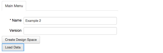
Again, the project can be verified by visiting the System tab in the top bar.
Co-localizing cases in a 1-D slice.
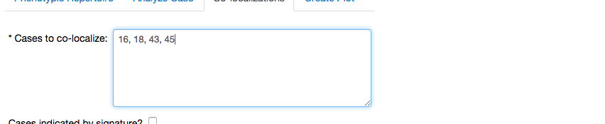
In the following example we will look at 4 cases of the design space of Example 2. The cases are Case 16, 18, 43 and 45 and have been chosen from a previous analysis of this model, which revealed that all four phenotypes have the potential to exhibit oscillatory behavior (Lomnitz, 2015). Here, we do not explore these phenotypes with the aim to identify the oscillatory phenotypes, but instead focus purely on the aspect of co-localization.
To co-localize these phenotypes, we select the Co-localizations tab of the Main Menu,
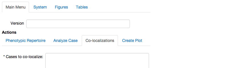
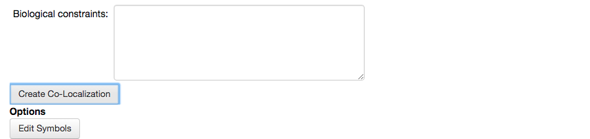
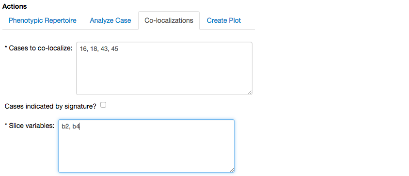
which expands a menu showing fields to define the cases we want to co-localize,
the slice varables for the co-localization, in this case we will utilize \(\beta_4\),
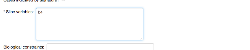
and the optional field to add bological constraints, which we leave empty.
We select the option to Create Co-localization,
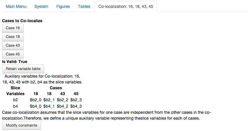
which adds a new tab in the top bar with the report for the co-localization,
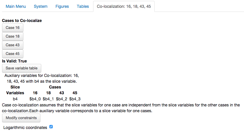
This new tab shows a wealth of information associated with the co-localization, which os broken down below:
The cases that were in the co-localized are shown as a list of buttons
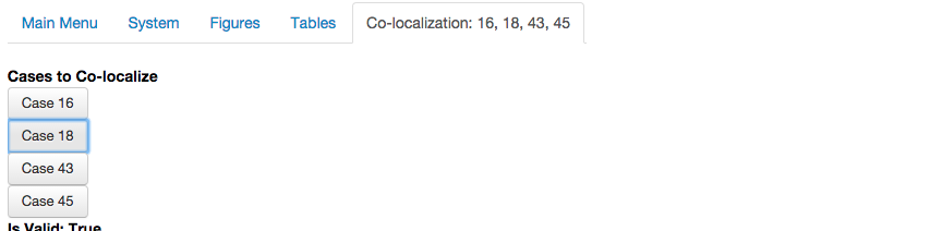
Each case can be selected, which opens the analysis report for that case. If the cases were succesfully co-localized, the case report is created with a pre-determined set of automatically determined values for the parameters. These parameter values are those for the co-localization.
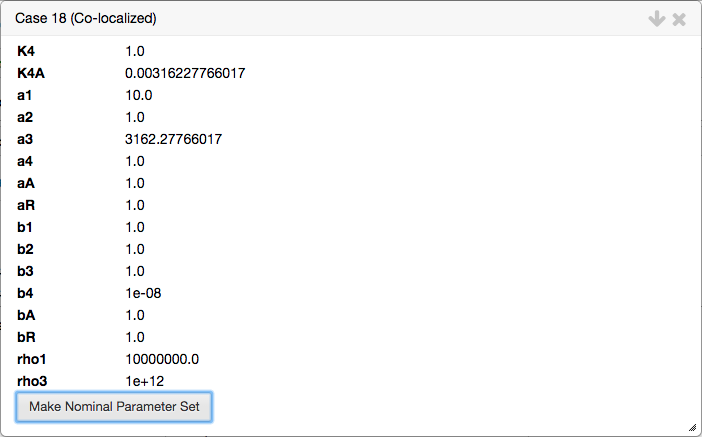
The values for the parameters for the selected case can be copied and stored in the internal parameter set using the
Make Nominal Parameter Setoption. We select the option to make this set of parameter values the nominal set, which will be used later in this section.The validity of the co-localization.

The table of auxiliary variables.

The option to modify constraints of the co-localization.

The details of this option will be seen later in the last sub-section.
The option to create a plot showing the co-localization (for 1D and 2D co-localizations only).
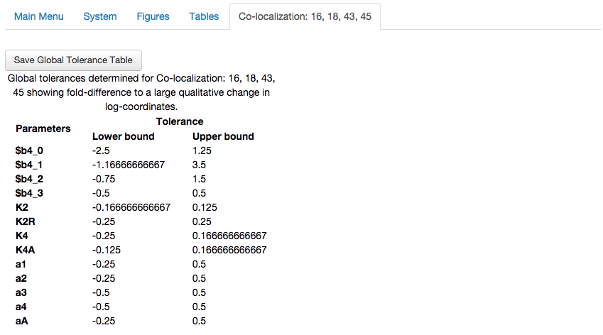
The global tolerance of the co-localization, showing the fold-difference required in each parameter for a qualitative change in system behavior.
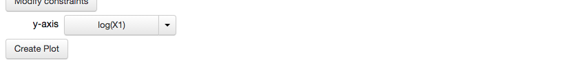
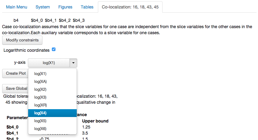
Next, we visualize the co-localization by creating a plot. Because this co-localization is a 1D plot, we will represent the slice variable on the x-axis and reprsent the steady-state concentration of one of the variables on the y-axis. By default, the plot will show the log of the concentration, but this can be changed to its arithmetic value by unchecking the Logarithmic coordinates option.
For this plot, we select the y-axis to be log(X4),
Create Plot option, which results in the following plot
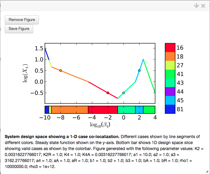
Note that this plot is created without setting the nominal values for the parameters. The range of the x-axis is selected automatically to include all the cases that were co-localized.
Using the Create Plot tab in the Main Menu, we can visualize other aspects of system behavior for this particular slice of design space. Recall that we set the internal parameter set to be equal to the parameter values automatically determined for Case 18 of this co-localization.
We select the Create Plot tab in the Main Menu and create a 1D plot by setting the Y-Axis variable to None. This allows us to plot 1D design spaces, 1D stability plots and 1D steady-state concentration, fluxes and functions.
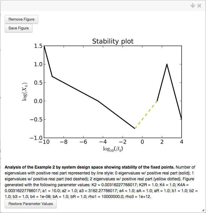
Here, we will show a 1D stability plot that is used to mimic 1D bifurcation diagrams. We set the * Plot Type to be equal to Stability, set the Y-Axis field to None (at which point the menu changes), set the range of the X axis to be that of the plot above, and set the new Y-Axis field to be equal to log(X4),
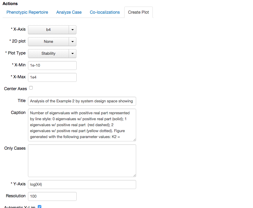
which yields the following 1D stability plot,
The analysis shown above can be repeated to show other co-localizations. For example, we create a co-localization using the same cases but with a different slice variable, e.g. \(\beta_2\). We enter the cases and slice variable in the corresponding fields of the Co-Localizations menu in the top bar,
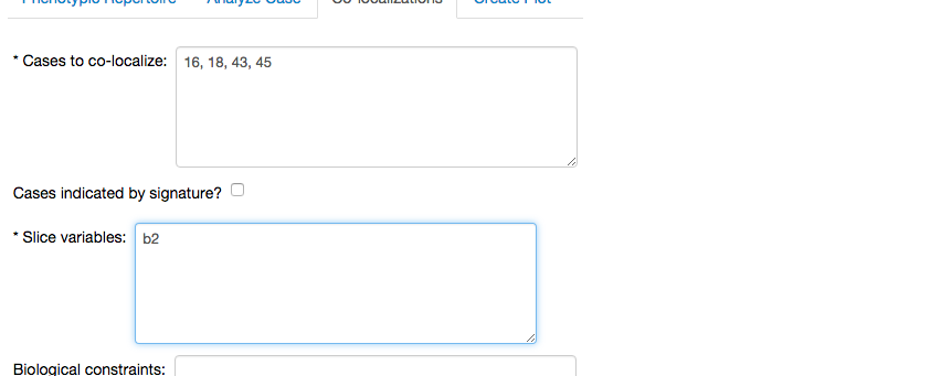
and select the Create Co-Localization option. We see a similar report to the one we obtaned with \(\beta_4\) as the slice variable, with some slight but very important differences,
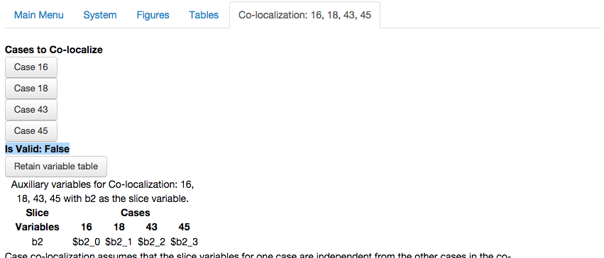
In this example, the co-localization was not valid. The implications of this is that there is no combination of parameter values such that cases 16, 18, 43, and 45 are simultaneously realized with \(\beta_2\) as the slice variable - regardless of values for the parameters. This shows the power of design space to exclude certain hypotheses on the basis of the model's lack of potential to generate specific progressions between phenotypes - regardless of values for the parameters.
Co-localizing cases in a 2-D and n-D slices.
The co-localizations have been limited to the 1D case involving single slice variable. However, co-localizations in higher dimensions can also be performed and the required steps to define them are the same as in the 1D case.
In the following example we will perform a 2D co-localization using the same cases as in the previous example, with \(\beta_2\) and \(\beta_4\) as the slice variables,
The result of the co-localization yields another co-localization report, with some subtle differences.
The co-localization report for a 2D co-localization shows the same basic information but in this case the table showing the auxiliary variables has 8 variables, instead of the 4 seen in the 1 D co-localizations. Also, the option to create a plot does not allow for a Y-Axis to be specified as the x and y axes will be the 2 slice variables we defined for the co-localization.
To visualize this co-localization, we select the Create plot options with the following result,
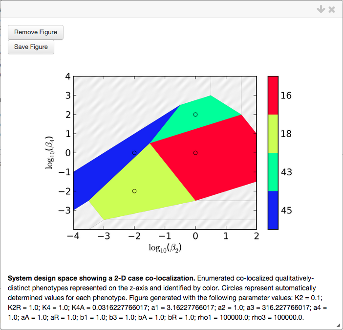
where only the co-localized cases are shown. Points are added to the plots showing the automatically determined values for the slice variables for each of the co-localized cases.
Co-localizations are not limited to the 1D and 2D case but can be extended for the \(n\)-th dimension by specifying \(n\) different slice variables. For example, we can co-localize case 16, 18, 43 and 45 in a 3D slice by specifying 3 slice variables, in this case \(\beta_2\), \(\beta_4\) and \(\beta_A\).
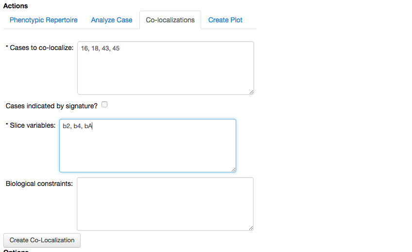
After selecting the Create Co-localization option, we get a new co-localization report showing the three slice variables and the corresponding auxiliary variables for each case, 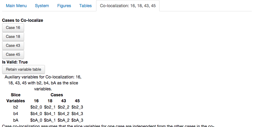
with similar results to the 1D and 2D co-localizations. Visualization of a 3D co-localization is possible (albeit this is experimental) by specifying the Create plot option,
Warning, 3D plots are experimental and have known bugs that may cause the program to crash. Progress should be saved prior to creating the 3D co-localization plot.
Creating the 3D plot for this co-localization yields the following plot,
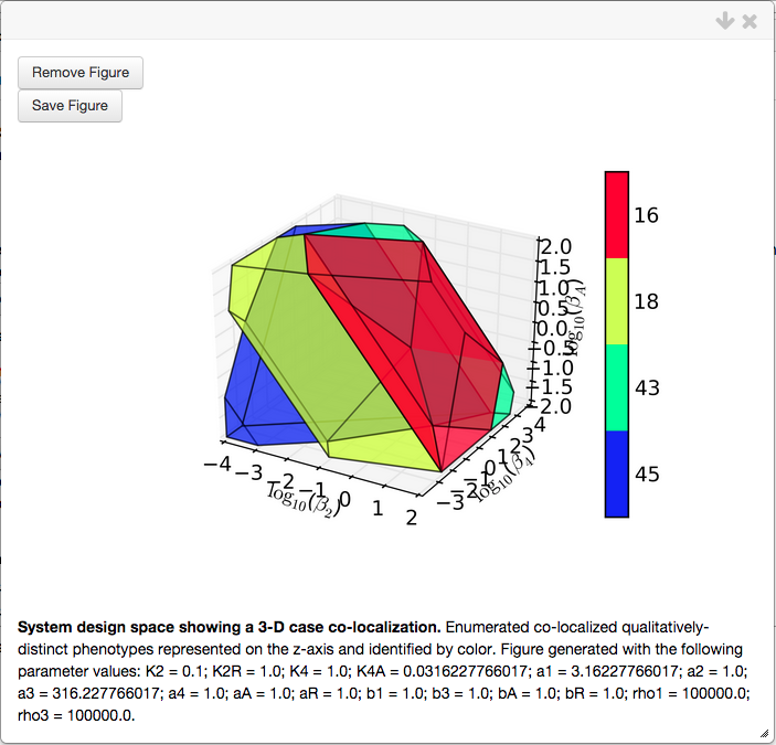
The \(n\)-D co-localization, where \(n > 3\), yields similar results as the 3-D case. The visualization of the co-localization in higher than 3 dimensions uses parallel co-ordinate plots to visualize the values for the slice variable of each case (not shown here).
Arranging cases for a specific behavior.
The co-localization of phenotypes is achieves by identifying \(k\) points, where \(k\) is the number of cases in the co-localization. Here, we show that by adding constraints to the co-localization, a slice of design space cam be obtained with a particular arrangement. These constraints may specify relationships between the auxiliary variables and between auxiliary variables and parameters of the system. This can be particularly useful if trying to determine if a particular progression of behaviors can be achieved as we increase some independent variable. In the 2D case, this can be useful to determine if phenotypes can be arranged relative to each other such that a certain landscape of behavior.
Here, we show an example using a 1D arrangment of phenotypes. To achieve this arrangement, we begin by creating a 1D co-localization for cases 34 and 45 with \(\beta_4\) as the slice variable,
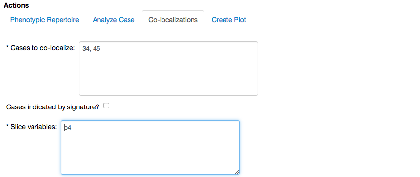
where case 34 is an unstable phenotype, as shown here, and 45 is one of the phenotypes co-localized in the previous sub-sections.
We select the option to create the co-localization, which yields the following report
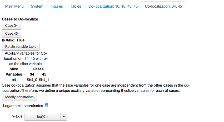
showing that the co-localization is valid, together with the other options discussed in the first subsection.
Up to this point, we have simply co-localized the phenotypes but not arranged them in any way. This co-localization can be visualized using the Create Plot option,
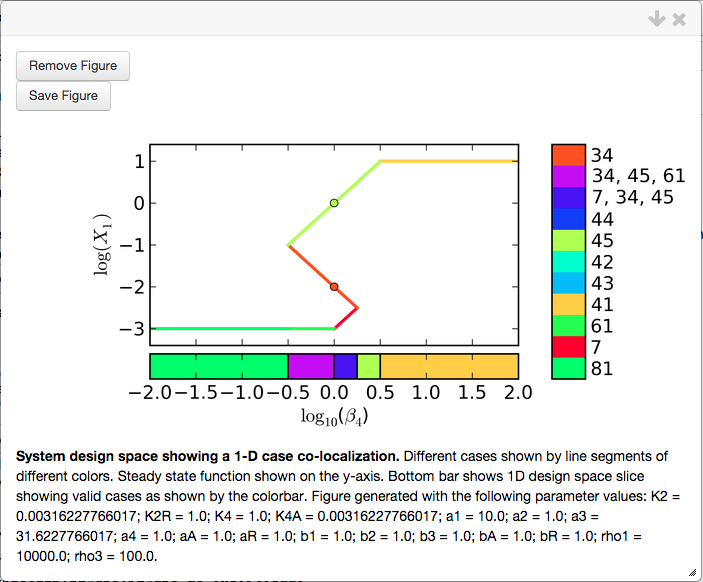
This co-localization will serve as a reference when shwoing the effects of arranging phenotypes. This particular figure shows an induction curve with a basal level of \(X_1\) for \(\beta_4 < 10^{-0.5}\), a maximal level of \(X_1\) for \(\beta_4 > 10^{0.5}\), and regions of overlap with 3 fixed points for \(10^{-0.5} < \beta_4 < 10^{0.5}\). Finally, the automatically determined points for the co-localized cases, 34 and 45, have the same value for the \(\beta_4\) parameter as shown by the orange and yellow/green dots, respectively.
But, what if we want the point for Case 34 to be left of the point for Case 45?
The design space toolbox can achieve this by imposing constraints on the auxiliary variables during co-localization by selecting the Modify Constraints option,
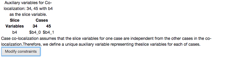
which adds a text field where we can specify relationships among the auxiliary variables and parameters of the model.
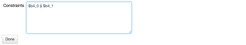
If we want the point for Case 34 to be to the left of the point for Case 45, then the auxiliary variable representing \(\beta_4\) for the point in Case 34 should be less than the auxiliary variable representing \(\beta_4\) for the point in Case 45, where $b4_0 and $b4_1 correspond to the \(\beta_4\) parameter for cases 34 and 45, respectively (as shown by the table above).
We enter the constraint in the text field
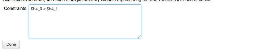
and select the Done option, which updates the Co-localization report. The results of arranging the phenotypes can be visualized by creating a new plot using the Create Plot option
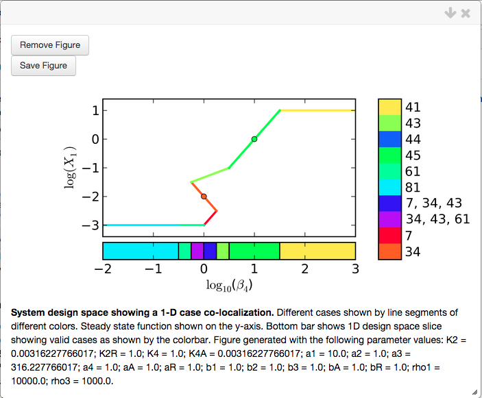
showing that indeed the point for Case 34 is to the left of the point for Case 45. We have shown that Case 34 can be to the left of Case 45, but can the reverse also be true? We Modify Constraints again and reverse the inequality,
select the Done option, and visualize the results using the Create Plot option

showing that the point for Case 34 is to the right of the point for Case 45.
Arranging Phenotypes with Minimum Sizes
We can also use the constraints options to specify the minimum width for a phenotypic region and a maximum separation between the co-localized points. To illustrate this, we define a new Co-localization for cases 34 and 45 with \(\beta_4\) as the slice variable.
In this example, the goal is to to have a minimum width of 100-fold for Case 34; a minimum width of 10-fold for Case 45; arrange the points such that Case 45 is to the right of Case 34; and finally, we will specify that all the points co-localized in this way will be within a space of 3 orders of magnitude.
To achieve these goals we duplicate each of the cases when defining the co-localization,
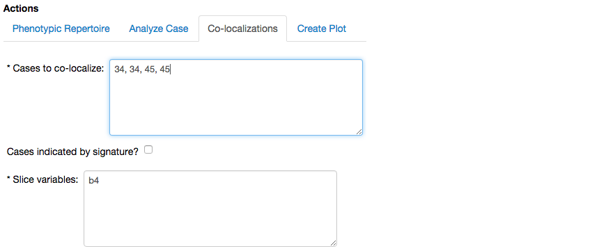
and select the Create Co-localization option, which yields the following report,
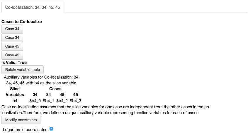
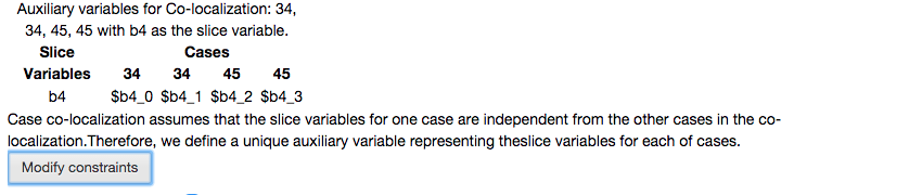
where cases 34 and 45 appear duplicated in the list of cases. They also appear duplicated in the table showing the auxiliary variables. However, note that each duplicate has its own Auxiliary variable that can be used to specify constraints between multiple points, in this case 2, within the same phenotypic region.
We select the Modify constraints option
and add constraints between the auxiliary variables. Recall that we want (1) Case 34 to be at least 100-fold wide ($b4_0 > 100*$b4_1); (2) Case 45 to be at least 10-fold wide ($b4_3 > 10*$b4_2); (3) the points for Case 45 be to the right of those for Case 34 ($b4_2 > $b4_0); and (4) all the values of the auxiliary variables to be within a span of 3 orders of magnitude ($b4_3 < 1001*$b4_1),
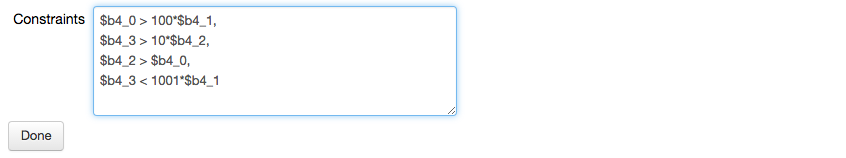
Note: constraints are imposed on individial points within a case, and not the entire phenotypic region.
We select the Done option, and visualize the co-localization using the Create Plot option,
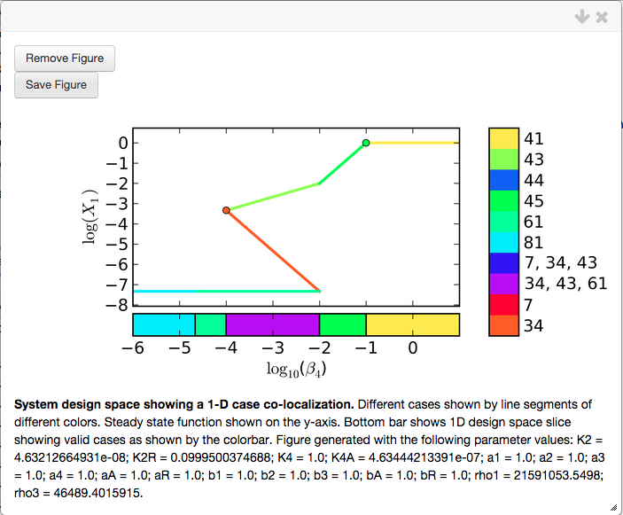
showing that the goal has been satsified. Case 34 (orange line) is 2-decades wide; Case 45 is 1 decade wide (bright green line); the entire phenotypic region for Case 34 is to the left of the phenotypic region of Case 45; and the phenotypic regions for cases 34 and 45 combined span a range of 3 decades.
The tools provided by the design space toolbox can be useful for determining if sets of parameter values exist such that a specific progression of behaviors is observed; or, alternatively if phenotypes satisfy certain requirements such as those pertaining to width and seperation. These tools can be useful to estimate parameters for natural systems, and to predict values for a synthetic system that would result in a desired behavior.
Jason G. Lomnitz
Savageau Lab
Department of Biomedical Engineering
University of California
Davis, CA 95616
jlomn@ucdavis.edu