Previous Section Table of Contents Next Section

Formulating a problem using the Design Space Toolbox

In this section, we show the details of formulating a model using the design space toolbox. We describe (1) key definitions of the design space method and model recasting into the Generalized Mass Action (GMA) form, (2) model input into the design space toolbox using a string representation of the equations, (3) architectural constraints during model formulation and (4) creating a design space project. In this section we will setup and save the design space project that will be used in the following sections.

Design space preliminaries: model formulation and recasting

The design space method identifies qualitatively-distinct phenotypes using a rigorous definition of phenotype based on the idea of term dominance (Savageau, 2009). A detailed definition of the key terminology has been recently reviewed (Lomnitz, 2015) and a brief version is provided here.

Architectural Features

The architectural features of a system are those that remain fixed independent of the parameter values that characterize particular instantiations of a system design. Important architectural features include (a) the network topology of interactions, (b) the signs of the interactions, and (c) the number of binding sites involved in the interactions.

Dominant Terms

The largest positive term in an equation we call the dominant positive term and the largest negative term in an equations we call the dominant negative term.

Dominant Sub-System

A dominant sub-system of the intact is where only dominant terms are retained, and all non-dominant terms are neglected. The result is a non-lineary system in the S-System form that has only one positive synthesis term and one negative degradation term.

Quantitative Phenotypes

Any state of a GMA system that is a fixed point, or steady-state of the system, we define as a quantitative phenotype of the system. A quantitative phenotype will have a positive term and a negative term in each equation that is larger than every other term of the given sign in that equation.

Qualitative Phenotypes

The infinite number of quantitative phenotypes have only a finite number of dominant S-systems, which suggests a natural grouping of phenotypes according to their dominant S-systems. A potentially valid qualitatively-distinct phenotype is defined by having a unique dominant S-system with a particular combination of dominant terms. However, not all combinations yield a valid phenotype: the nonlinear S-Systems that represent the qualitatively-distinct phenotypes may not have a steady-state solution, alternatively the boundary conditions that determine the region of validity may not be satisfied anywhere in design space. A qualitatively-distinct phenotype is defined as a potentially valid one that has been determined to be valid.

Phenotypic Repertoire

The Phenotypic repertoire is defined as the collection of qualitatively-distinct phenotypes integrated into the space-filling structure called the system design space (Savageau, 2009; Lomnitz, 2013).

Mathematical Model

For the purpose of illustration, we use the model of a synthetic gene circuit design that has been shown to exhibit sustained oscillations (Lomnitz, 2014). This example is chosen because it is relatively simple and it exhibits rich behaviors that include oscillations, hysteresis and different input-output couplings. The general strategy that will be used to analyze this model involves an automated strategy that does not require prior knowledge of the values for the parameters (Lomnitz, 2015).

The model represents a transcriptional gene circuit involving two regulators, an activator and a repressor, that are coupled using both positive and negative feedback loops. The activator activates its own synthesis and activates the synthesis of a repressor. The repressor in turn represses synthesis of the activator and that of its own synthesis. The mathematical model for this circuits is given by the following system of first order differential equations,

\(\frac{dX_1}{dt} = \alpha_1 \left[\frac{1 + \left(X_2/K_2\right)^{g_{12}} + \rho_1^{-1}\left(X_4/K_{4A}\right)^{g_{14}}}{1 + \left(X_2/K_2\right)^{g_{12}} + \left(X_4/K_{4A}\right)^{g_{14}}}\right] - \beta_1 X_1 - \mu X_1\) \(\frac{dX_A}{dt} = \alpha_AX_1 - \beta_A X_A - \mu X_A\) \(\frac{dX_2}{dt} = \alpha_2X_A - \beta_2 X_2 - \mu X_2\) \(\frac{dX_3}{dt} = \alpha_3 \left[\frac{\rho_3^{-1} + \left(X_2/K_{2R}\right)^{g_{32}} + \rho_3^{-1}\left(X_4/K_4\right)^{g_{34}}}{1 + \left(X_2/K_{2R}\right)^{g_{32}} + \left(X_4/K_4\right)^{g_{34}}}\right] - \beta_1 X_1 - \mu X_1\) \(\frac{dX_R}{dt} = \alpha_RX_3 - \beta_R X_R - \mu X_R\) \(\frac{dX_4}{dt} = \alpha_4X_R - \beta_4 X_4 - \mu X_4\)

where \(X_1\), \(X_A\) and \(X_2\) represent the concentration of activator mRNA, immature regulator and mature regulator, respectively; \(X_3\), \(X_R\) and \(X_4\) represent the concentration of repressor mRNA, immature regulator and mature regulator, respectively; \(\alpha_i\), where \(i = \left\{1, 3\right\}\), represents the maximum level of activator and repressor transcription, respectively; \(\alpha_i\), where \(i = \{A, 2\}\), represents the first order rate constant for synthesis of the immature and mature form of the activator, respectiely; \(\alpha_i\), where \(i = \{R, 4\}\), represents the first order rate constant for synthesis of the immature and mature form of the repressor, respectiely; \(\beta_i\), where \(i = \{1, A, 2, 3, R, 4\}\), represents the first order rate constant for loss due to active degradations for the \(X_i\) species; \(\rho_i > 1\), where \(i = \{1, 3\}\) represents the fold difference between maximal and basal rate of transcription of the \(X_i\) species; \(\mu\) represents the rate of loss by dilution due to exponential growth. The \(K_2\) and \(K_{2R}\) parameters represent the concentration of activator for half-maximal activation of the activator and repressor mRNA, respectively. The \(K_{4A}\) and \(K_4\) parameters represent the concentration of repressor for half-maximal repression of the activator and repressor, respectively; The \(g_{ij}\) parameters represent the number of sites for binding by the \(X_j\) species to the promoter of the gene encoding the \(X_i\) mRNA molecule (Lomnitz, 2014).

It should be noted that there are constraints in the definitions of certain parameters of the model. Here, the \(\rho_1\) and \(\rho_3\) parameters are defined strictly greater than 1, otherwise they would represent a completely different mechanism (i.e. repression instead of activation, or vice versa). Other important examples of architectural constraints are the kinetic orders which must be defined as constants and not symbols. Here, the \(g_{ij}\) kinetic orders are defined to be equal to 2. This example system is used here because (1) it is a relatively simple system, (2) it can exhibit interesting induction characteristics, (3) it must be recast into the standard GMA form - required by the design space method - and (4) there are architectural constraints that must be explicitly defined.

In addition, we simplify the model by assuming that \(\mu < \beta_i\) for all \(i = \{1, A, 2, 3, R, 4\}\). This assumption in design space means that the last term for each of the equations can never be dominant, and thus we remove them from the equations. These terms need not be removed explicitly; instead, we can define additional architectural constraints that achieve the same effect. By removing them from the model we reduce the number of cases and simplifies the model thus facilitating illustration of the toolbox.

Recasting the system into the GMA form

In order to apply the design space methodology, we recast the model into the generic GMA form. This can be done exactly by following a defined series of steps (Savageau, 1987). For most biochemical systems, the recasting process into the GMA form is fairly straight forward. Using the example system we previously described, we show the steps typically needed for recasting rational functions to the GMA form.

The steps to recast most biochemical systems typically involves

Expanding the terms in the numerator by multiplying through by common factors.
Defining auxiliary variables for each denominator with multiple terms.
Substituting denominators by the corresponding auxiliary variables.
Defining a new system involving the modified equations and the equations for the auxiliary variables.

Example of Recasting

Step 0. Original system [note: the last negative term in each equation has been removed].

\(\frac{dX_1}{dt} = \alpha_1 \left[\frac{1 + \left(X_2/K_2\right)^{g_{12}} + \rho_1^{-1}\left(X_4/K_{4A}\right)^{g_{14}}}{1 + \left(X_2/K_2\right)^{g_{12}} + \left(X_4/K_{4A}\right)^{g_{14}}}\right] - \beta_1 X_1\) \(\frac{dX_A}{dt} = \alpha_AX_1 - \beta_A X_A\) \(\frac{dX_2}{dt} = \alpha_2X_A - \beta_2 X_2\) \(\frac{dX_3}{dt} = \alpha_3 \left[\frac{\rho_3^{-1} + \left(X_2/K_{2R}\right)^{g_{32}} + \rho_3^{-1}\left(X_4/K_4\right)^{g_{34}}}{1 + \left(X_2/K_{2R}\right)^{g_{32}} + \left(X_4/K_4\right)^{g_{34}}}\right] - \beta_3 X_3\) \(\frac{dX_R}{dt} = \alpha_RX_3 - \beta_R X_R\) \(\frac{dX_4}{dt} = \alpha_4X_R - \beta_4 X_4\)

Step 1. Expanding numerators of the equations for \(X_1\) and \(X_3\) by multiplying through by the \(\alpha\) parameters.

\(\frac{dX_1}{dt} = \frac{\alpha_1 + \alpha_1X_2^{g_{12}}K_2^{-g_{12}} + \alpha_1\rho_1^{-1}X_4^{g_{14}}K_{4A}^{-g_{14}}}{1 + X_2^{g_{12}}K_2^{-g_{12}} + X_4^{g_{14}}K_{4A}^{-g_{14}}} - \beta_1 X_1\) \(\frac{dX_3}{dt} = \frac{\alpha_3\rho_3^{-1} + \alpha_3X_2^{g_{32}}K_{2R}^{-g_{32}} + \alpha_3\rho_3^{-1}X_4^{g_{34}}K_4^{-g_{34}}}{1 + X_2^{g_{32}}K_{2R}^{-g_{32}} + X_4^{g_{34}}K_4^{-g_{34}}} - \beta_3 X_3\)

Step 2. Defining auxiliary variables, \(X_5\) and \(X_6\), defined as the expressions in the denominators of the first and second synthesis terms,

\(X_5 = 1 + X_2^{g_{12}}K_2^{-g_{12}} + X_4^{g_{14}}K_{4A}^{-g_{14}}\) \(X_6 = 1 + X_2^{g_{32}}K_{2R}^{-g_{32}} + X_4^{g_{34}}K_4^{-g_{34}}\)

Step 3. Substituting auxiliary variables into the original equations.

\(\frac{dX_1}{dt} = \alpha_1X_5^{-1} + \alpha_1X_2^{g_{12}}K_2^{-g_{12}}X_5^{-1} + \alpha_1\rho_1^{-1}X_4^{g_{14}}K_{4A}^{-g_{14}}X_5^{-1} - \beta_1 X_1\) \(\frac{dX_3}{dt} = \alpha_3\rho_3^{-1}X_6^{-1} + \alpha_3X_2^{g_{32}}K_{2R}^{-g_{32}}X_6^{-1} + \alpha_3\rho_3^{-1}X_4^{g_{34}}K_4^{-g_{34}}X_6^{-1} - \beta_3 X_3\)

Step 4. Defining a new system by adding the algebraic constraints.

\(\frac{dX_1}{dt} = \alpha_1X_5^{-1} + \alpha_1X_2^{g_{12}}K_2^{-g_{12}}X_5^{-1} + \alpha_1\rho_1^{-1}X_4^{g_{14}}K_{4A}^{-g_{14}}X_5^{-1} - \beta_1 X_1\) \(\frac{dX_A}{dt} = \alpha_AX_1 - \beta_A X_A\) \(\frac{dX_2}{dt} = \alpha_2X_A - \beta_2 X_2\) \(\frac{dX_3}{dt} = \alpha_3\rho_3^{-1}X_6^{-1} + \alpha_3X_2^{g_{32}}K_{2R}^{-g_{32}}X_6^{-1} + \alpha_3\rho_3^{-1}X_4^{g_{34}}K_4^{-g_{34}}X_6^{-1} - \beta_3 X_3\) \(\frac{dX_R}{dt} = \alpha_RX_3 - \beta_R X_R\) \(\frac{dX_4}{dt} = \alpha_4X_R - \beta_4 X_4\) \(X_5 = 1 + X_2^{g_{12}}K_2^{-g_{12}} + X_4^{g_{14}}K_{4A}^{-g_{14}}\) \(X_6 = 1 + X_2^{g_{32}}K_{2R}^{-g_{32}} + X_4^{g_{34}}K_4^{-g_{34}}\)

Toolbox input: model equations and architectural constraints

As in the previous section, the first step is to import the interactive widgets into the ipython notebook environment,

from dspace.display.UI.interactive_input import InteractiveInput

Mathematical models in string representation

The design space toolbox has a built-in computer algebra system that is responsible for representing mathematical expression internally. Once represented internally, it carries out operations that include symbolic algebraic manipulations and numerical evaluation of mathematical functions.

The computer algebra system enables mathematical models in the GMA-form to be directly input into the design space toolbox by their string representation. For the strings to be parsed by the algebra system, they must abide by the following rules:

Variable names must start with an alphabetical character, and are comprised of alphanumeric character or underscores.
Constants may be expressed as integers, decimal numbers or using scientific notation.
The differential operator is . according to Newton notation (i.e. \(dx/dt\) \(\equiv\) \(\dot{x}\)).
Operators must be made explicit (i.e., 3*x is allowed, 3x is not).
The supported operators are:
- Differential: . (e.g., x. = 0 represents \(\dot{x} = 0\))
- Sum: +
- Substraction: -
- Multiplication: *
- Division: /
- Power: ^
- Equals: =
- Less Than: <
- Greater Than: >
The left-hand side of an equation must be a differentiated variable, an auxiliary variable or 0 (in which case auxiliary variable must be explicitly stated).
The right-hand side of all the equations must be sums of products of power-laws (division is allowed instead of inverse power).
The left-hand side and right-hand side of an inequality are treated equally.

Using the above rules, we represent the system of equations for the recast model above by the following list of strings,

recast_model = ['X1. = a1*X5^-1 + a1*X2^g12*K2^-g12*X5^-1 + a1*rho1^-1*X4^g14*K4A^-g14*X5^-1 - b1*X1',
                'XA. = aA*X1 - bA*XA',
                'X2. = a2*XA - b2*X2',
                'X3. = a3*rho3^-1*X6^-1 + a3*X2^g32*K2R^-g32*X6^-1 + a3*rho3^-1*X4^g34*K4^-g34*X6^-1 - b3*X3',
                'XR. = aR*X3 - bR*XR',
                'X4. = a3*XR - b4*X4',
                'X5 =  1 + X2^g12*K2^-g12 + X4^g14*K4A^-g14',
                'X6 =  1 + X2^g32*K2R^-g32 + X4^g34*K4^-g34',
                ]

Definition of Architectural Constraints

Constraints on the parameters

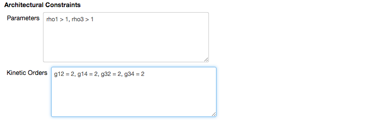
The architectural features of a system are those that remain fixed independent of specific values for the parameters. In this model, we have that the parameters \(\rho_1\) and \(\rho_3\), which represent potential capacity for activation and repression of \(X_2\) and \(X_4\), respectively, be larger than 1. These constraints are represented using the followng string notation,

architectural_paramaters = ['rho1 > 1',
                            'rho3 > 1']

It should be noted that more complex architectural constraints for the system parameters may also be defined. The design space toolbox accepts constraints as long as both sides of the inequality are positive products of power-laws.

Constraints on the kinetic orders

For this mathematical model we have defined variable kinetic orders represented by the symbols \(g_{12}\), \(g_{14}\), \(g_{32}\) and \(g_{34}\). The design space toolbox requires that all kinetic orders be defined by constant values. The specific values of the kinetic orders alter the mechanism by which different components are binding and thus their values are considered to be architectural. Here, we assume that binding occurs with a cooperativity of 2, such that \(g_{12} = g_{14} = g_{32} = g_{34} = 2\). These constraints on the kinetic orders are represented by the following string representations,

architectural_kinetic_orders = ['g12 = 2',
                                'g14 = 2',
                                'g32 = 2',
                                'g34 = 2']

Mathematical typesetting of equations in string representation

The IPython notebook provides a document-like format that integrates code execution, formatted text, mathematical expressions, figures and other digital media. The design space toolbox integrates with the IPython notebook to display typeset mathematical expressions. This is achieved by automatically representing expressions using latex notation. The latex representation for symbols in the model are provided as key-value pairs. For example, X1 in the string representation of the model represents the symbol \(X_1\); the latex representation of \(X_1\) is X_1, thus the key-value pair is

'X1':'X_1'

The key-value pairs for all the symbols of the model are defined in a dictionary, which in his case is the following,

latex_symbols = {'X1':'X_1',
                 'X2':'X_2',
                 'X3':'X_3',
                 'X4':'X_4',
                 'XA':'X_A',
                 'XR':'X_R',
                 'X5':'X_5',
                 'X6':'X_6',
                 'a1':r'\alpha_{1}',
                 'a2':r'\alpha_{2}',
                 'a3':r'\alpha_{3}',
                 'a4':r'\alpha_{4}',
                 'aA':r'\alpha_{A}',
                 'aR':r'\alpha_{R}',
                 'b1':r'\beta_{1}',
                 'b2':r'\beta_{2}',
                 'b3':r'\beta_{3}',
                 'b4':r'\beta_{4}',
                 'bA':r'\beta_{A}',
                 'bR':r'\beta_{R}',
                 'mu':r'\mu',
                 'K2':'K_2',
                 'K2R':'K_{2R}',
                 'K4':'K_4',
                 'K4A':'K_{4A}',
                 'rho1':r'\rho_1',
                 'rho3':r'\rho_3',
                 }

Creating a system design space object

With the model and constraints defined in their string representation, we can proceed to create a new design space project using the graphical widget component. The focus of this sub-section is to provide an overview of the widget user interface.

To initiate the widgets, we create a new InteractiveInput object. The InteractiveInput object is created with multiple optional arguments (e.g., equations=simple_model) that populate default values of different fields. The fields that are populated by different arguments will be discussed as they become relevant.

simple_example_widget=InteractiveInput(name='Example 2',
                                       equations=recast_model,
                                       auxiliary_variables=['X5', 'X6'],
                                       constraints=architectural_paramaters,
                                       kinetic_orders=architectural_kinetic_orders,
                                       symbols=latex_symbols)

We run the previous cell and start with the main menu shown in Section I. However, note that the Name field is populated by the value indicated by the name='Example 2' keyword argument,

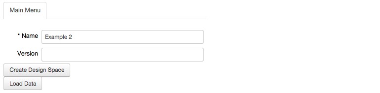
By selecting the Create design space option, the main meny expands to show the fields to define the model for the design space project. However, this time we see many of the fields have been populated.

The equations=recast_model option sets the default value of the Equations field to the system equations, including the algebraic constraints obtained by recasting, stored in the variable recast_model assigned here.

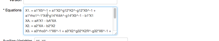
The auxiliary_variables=['X5', 'X6'] sets the default value for the auxiliary variables we defined during recasting, that are made explicit in the Auxiliary variables field.

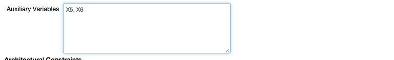
It should be noted that in this example the auxiliary variables do not have to be defined explicitly. This is because the equations for the algebraic constraints have the auxiliary variables on the left-hand side of the equations. The design space toolbox identifies these variables and implicitly defines them as the auxiliary variables.

The constraints=architectural_parameters sets the default value for the Parameters field of the Architectural Constraints subheading stored in the architectural_parameters variable assigned here.

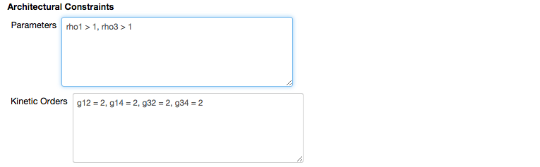
and the kinetic_orders=architectural_kinetic_orders sets the values for the Kinetic orders to the value stored in the architectural_kinetic_orders variable assigned here.

The remaining options of the menu for design space creation are used to make the design space perform additional analyses.

The Check for Cycles option is used to resolve systems that have cycles. These systems have possible combinations of dominant terms that lead to an underdetermined system, and the state of the system depends on sub-dominant fluxes. An example of a system that has this problem is shown by the diagram below,

where larger arrows are represented dominant fluxes. The dominant terms for this model would lead to the situation where A depends on C, which depends on B, which depends on A and thus there is an infinite number of solutions, called a solution subspace. However, this particular system does not have an infinite number of solutions. The system reaches a rapid equilibrium, and the state of the system is determined by the net flux into and out of the cycle pool. In this example, design space resolves this issue by including sub-dominant fluxes into and out of A.

The last option, to Check for Co-dominance, is used to resolve situations where two or more terms in an equations are, by definition, mathematically equivalent at steady state. An example of a system that has this problem is shown by the diagram below,

where, at steady state, the the two fluxes out of A are equal, thus the two fluxes into B are by definition equal as well and thus there cannot be a dominant flux into B.

Selecting the options to resolve cycles or co-dominance can add significant overhead when creating a design space, and thus should be avoided unless necessary. Furthermore, there can be overlap between cycles and co-dominance and thus they should not be used together as they can lead to anomalous results - again, unless absolutely necessary. After all these fields have been populated accordingly, and the options needed for the particular problem selected, we select the Done button.

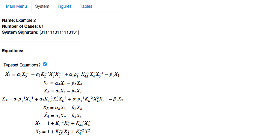
At this point it is best to verify the system is correct by visiting the System tab in the top bar, which should show the name Example 2 of the project, a total of 81 cases, and a system signature of [3111113111113131]. The model equations can be verified, which should be typeset with the symbols defined,

We finish this section by saving the project using the Save data button under Options in the Main Menu tab. This project will be used for each of the sections that follow.

Previous Section Table of Contents Next Section

Jason G. Lomnitz
Savageau Lab
Department of Biomedical Engineering
University of California
Davis, CA 95616
jlomn@ucdavis.edu