Previous Section Table of Contents Next Section

Enumerating the Phenotypic Repertoire

In this section we show the details of analyzing qualitatively-distinct phenotypes and enumerating the complete phenotypic repertoire of a model. We discuss (1) enumerating the complete repertoire of qualitatively-distinct phenotypes of a model, (2) qualitatively-distinct phenotypes and their dominant sub-systems, and (3) the phenotypic characterstics of phenotypes at the global level of the phenotypic repertoire. Here, we show how the design space toolbox can achieves this and how it can be used to gain understanding of the possible behaviors a model can exhibit from a global perspective.

IPython Notebook Preamble

This section, and every section after it, uses the model saved at the end of Section II. Because each section uses a new notebook, we import the interactive widgets into the ipython notebook environment,

from dspace.display.UI.interactive_input import InteractiveInput

and create a new interactive widget with the name of the widget saved in Section II.

simple_example_widget=InteractiveInput(name='Example 2')

and select the Load Data button,

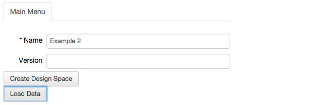
Again, the project can be verified by visiting the System tab in the top bar.

Enumerating the phenotypic repertoire, and its subsets.

The design space method provides a rigorous definition of phenotype that is purely a function of the structure of the mathematical equations. Because of this, the complete repertoire of possible phenotypes latent in a particular design can be enumerated, without specifying any values for the parameters. The task of enumerating the phenotypic repertoire is made simple using the design space toolbox. To do this, we visit the first tab in the Actions sub-menu under the Main Menu tab in the top bar,

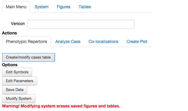
once the Phenotypic Repertoire tab has been selected, we see an expanded sub-menu with a single option: Create/modify cases table. This button allows us to create a table showing

1. All the potentially valid qualitatively-distinct phenotypes, the Cases of the model.
2. The set of Valid qualitatively-distinct phenotypes, i.e. the phenotypic repertoire.
3. A subset of User Specified cases.

The most useful of these options when analyzing a model from a global perspective is to select the option to view the Valid phenotypes. This option tells the program to enumerate the phenotypic repertoire, which becomes visible by selecting the Done option.

Note: for larger systems, enumerating the phenotypic repertoire may be time consuming. To determine if the toolbox is busy processing information, look at the top right corner for a solid black circle; otherwise, the if the circle is white with a black outline the toolbox is not busy.

The result of enumerating the phenotypic repertoire is a table showing each unique phenotype by its two unique identifiers, the Case Number and the Case Signature,

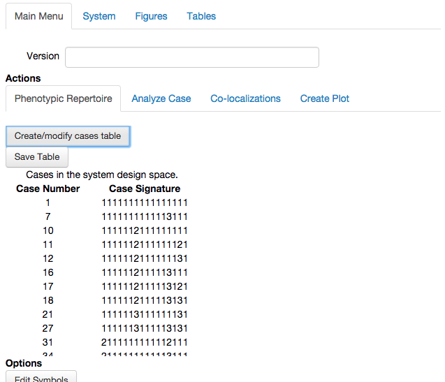
where the Case Number is a unique number for each case determined by arbitrarily enumerating the cases; and the Case Signature is constructed by identifying the index of the dominant positive and dominant negative terms for each equation of the full system in order that define the dominant S-System.

The table can be saved using the Save Table button above, in which case a copy of the table is popped out and is accesible under the Tables tab in the top bar and saves the current project according to its name and version number.

Once under the Tables tab, tables are saved to the project file when the Save Data option is selected in the Main Menu tab.

Note that when creating the table there was the option to add additional columns; this option will be revisited later in this section.

Qualitatively distinct phenotypes and their dominant S-systems

The table from the previous table shows the complete phenotypic repertoire of a system. However, this information by itself may not be very meaningful and thus the result may appear uneventful. Here, we add some context to the implications of enumerating the phenotypic repertoire by exploring the large amounts of information that this provides. In particular, we discuss the analysis of qualitatively-distinct phenotypes and explores some of the properties of the phenotypes that the design space toolbox makes readily available.

Qualitatively Distinct Phenotypes of a System

Each phenotype of the system is characterized by having a unique dominant sub-system, where the equations of the sub-system are in the S-system form (Savageau, 2009). The S-system form is a non-linear system for which there is an analytical solution for the steady states, which is obtained by transforming the steady-state equations to logarithmic coordinates. The system becomes linear in the logarithm of the variables and thus the system can be solved using linear analysis (Savageau, 1976). S-System analysis has been the focus of much research (Voit, 2013), which may be applied for analysis of qualitatively-distinct phenotypes of the system.

The design space toolbox provides a lot of information for each Case. This functionality is available under the Analyze Case tab in the Actions sub-menu of the Main Menu. Selecting the Analyze Case tab opens up the following expended menu,

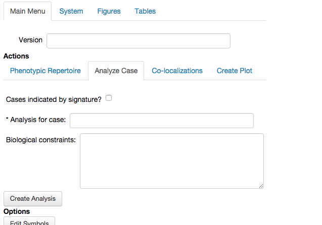
the required field in this menu is used to indicate the Case of the model that is to be analyzed. The case can be indicated either by its Case Signature, or by its Case Number. Although the Case Signature is more informative, we will use the Case Number because it is more convenient. The Case Number can be related to the Case Signature using Table 1.

As an optional field, we can define biological constraints that limit the analysis to a specific domain in the parameter and variables (dependent and independent) space. The details of imposing biological constraints will not be shown in this section.

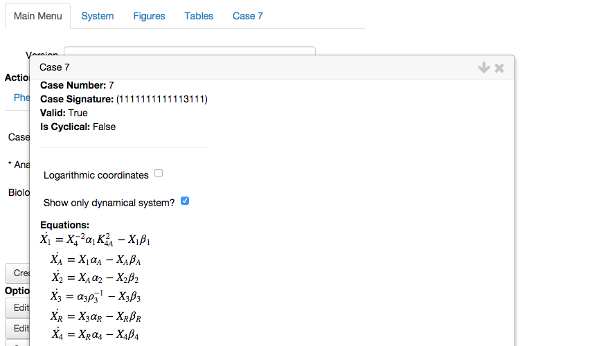
In this example, we choose the second case in Table 1, Case 7, which we enter in the Analysis for case field and leave the Biological constraints field empty. We select the Create Analysis option, which creates a new tab in the top bar and pops-up a widget with the analysis report for Case 7. This report shows basic information about the case from a global perspective and is independent of specific values for the parameters:

1. Case signature and Case number:

   
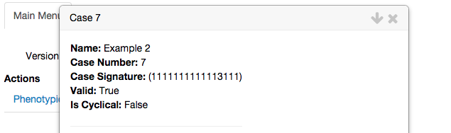
   As discussed earlier, the Case Signature represents the index of the positive term and the index of the negative term that is dominant for each equation of the full system in order. These dominant terms are used to define the dominant sub-system of the qualitatively-distinct phenotype.
   

2. The dominant sub-system equations:

   
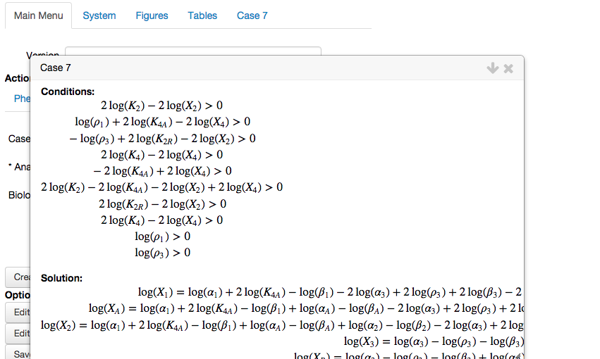
   The dominant sub-system is obtained from the Case Signature by retaining the dominant terms and neglect the non-dominant terms. The end result is a system with one positive term and one negative term, thus a system in the S-System form.
   

3. The conditions for the dominant sub-system to be consistent:

   
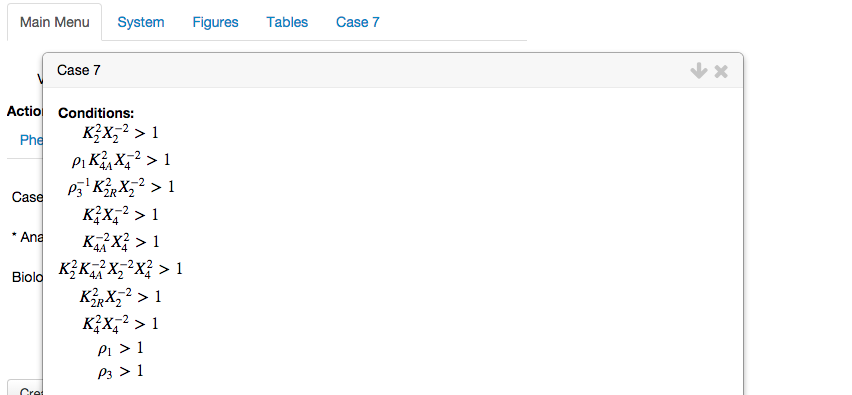
   After picking a dominant term, be it positive or negative, we are assuming that it is larger than every other term with the same sign in that equation. These assumptions are made explicit in these conditions of validity, that must be satisified for the dominance assumption to be valid.
   

4. The steady-state solution:

   
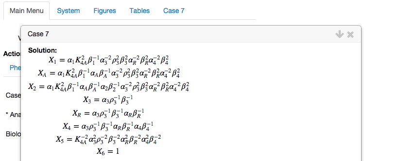
   The dominant sub-system can be solved for its steady-state solution, which the design space toolbox does automatically.
   

5. The boundaries obtained by substituting the steady-state solution into the conditions for validity:

   
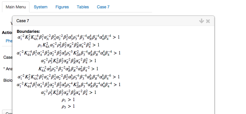
   The boundaries in parameter space that delimit the subspace within which a qualitatively distinct phenotype is valid are obtained by substituting in the steady-state solutions into the conditions of validity. The result is purely a function of parameters and independent variables.
   

6. The table showing all logartithmic gains and parameter sensitivities:

   
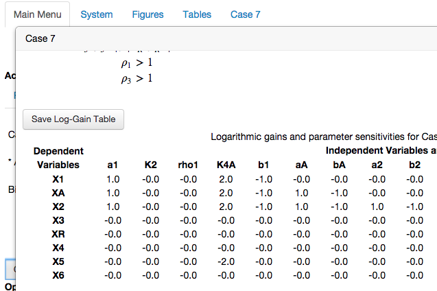
   The table of logarithmic gains for signal amplification factors indicate the change of a dependent variable in response to small changes in an independent variable. In the context of design space, independent variables and parameters are treated equally and thus this table shows log-gains and parameter sensitivities for local robustness.
   

7. The bounding box within which it is valid:

   The bounding box indicates the absolute values for the parameters that can be used such that the phenotype may still be valid. In high dimensional spaces, it is not uncommon for the bounding box to have values of ±∞, which indicate that any value of that parameter can be chosen such that there is a combination of values of the remaining parameters resulting in the validity of that phenotype.
   

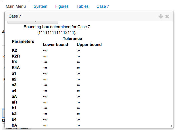
In addition, the equations for the dominant S-System can be expressed purely as a dynamical system,

and the conditions, solution, boundaries and the bounding box values can be automatically transformed to logarithmic coordinates,

Global-level analysis of the repertoire of phenotypic characteristics

The ability to look at each Case provides a wealth of information; however, it would be useful to inspect the repertoire of local behaviors, such as log-gains for a particular variable, of the entire phenotypic repertoire. For example, we might be interested in how \(X_4\) in each phenotype responds to a change in critical parameters such as \(\beta_2\) and \(\beta_4\).

The toolbox facilitates this by allowing columns to be aded to the phenotypic repertoire table. We modify the table showing the valid cases in the Phenotypic Repertoire menu of the the Main Menu tab by selecting the Create/modify cases table button. This expands the menu as shown previously. We then select the option to Add column,

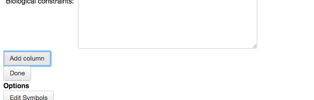
which displays additional field to add information to a new column.

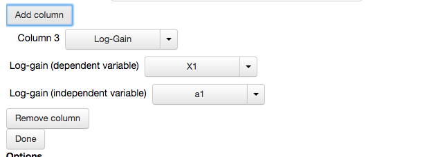
by default, the new column will show the logarithmic gain of \(X_1\) with respect to \(\alpha_1\). We change the dependent variable and independent variable fields to show the logaritmic gain of \(X_4\) with respect to \(\beta_2\). In addition, we add 2 more columns, where Column 4 will display the logaritmic gain of \(X_4\) with respect to \(\beta_4\) and column 5 will display the stability of a representative fixed point by showing the number of eigenvalues with positive real part,

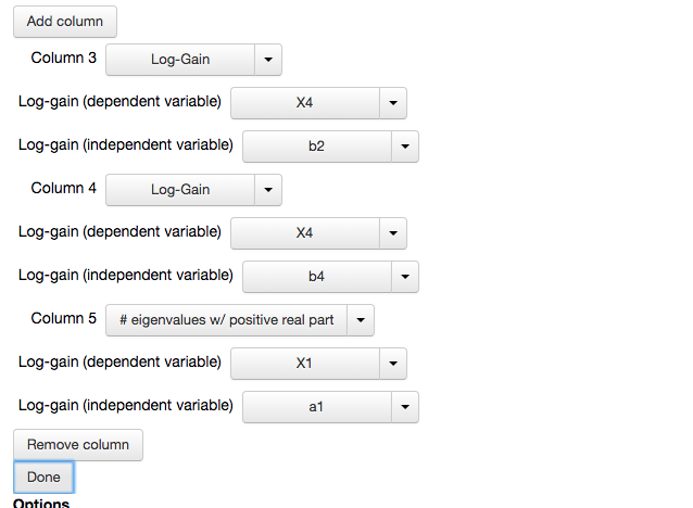
We select the Done option, which yields the following table,

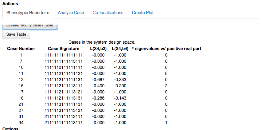
Note that for the stability of the fixed point to be determined, the design space toolbox needs to find a representative point within the phenotypic region. The design space toolbox is capable of determining values within the region of validity for any phenotype of the system, as will be shown in the next section.

In this example, we see one phenotype with 1 eigenvalue with positive real part denoting exponential instability, and one phenotype with 2 eigenvalues with positive real part consistent with limit cycle oscillations. It is important to reiterate that we have not specified values for any of the parameters and this analysis has been performed without prior knowledge of what the values for the parameters might be.

The ability to enumerate the phenotypic repertoire and explore the repertoire of potential behaviors in a model allows critical behaviors to be readily identified and helps focus computational efforts and analyses to specific localized regions of parameter space. This can be very useful when studying natural systems and when rationally engineering synthetic constructs intended to exhibit particular behaviors.

Previous Section Table of Contents Next Section

Jason G. Lomnitz
Savageau Lab
Department of Biomedical Engineering
University of California
Davis, CA 95616
jlomn@ucdavis.edu