Determining parameter values for Cases
This section focuses on the task of automatically determining values for any of the phenotypes of the model. Here we discuss (1) determining a representative set of parameter values for the parameters both at the architectural level and biological level, (2) performing local analyses such as local stability of the fixed points and looking at steady-state values and fluxes, and (3) quantifying the global tolerance defined as the fold-difference required in a parameter for large, qualitative changes in behavior.
IPython Notebook Preamble
We import the interactive widgets into the ipython notebook environment,
from dspace.display.UI.interactive_input import InteractiveInput
and load the example from Section III in the same way as we did in the previous section,
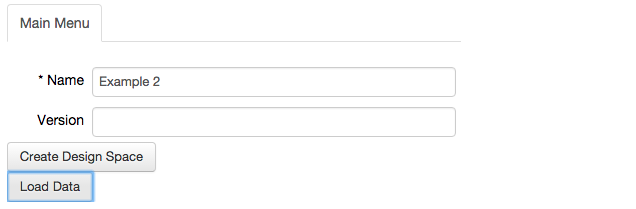
simple_example_widget=InteractiveInput(name='Example 2')
and select the Load Data button,
Again, the project can be verified by visiting the System tab in the top bar.
Automatically determined values for the parameters.
The design space toolbox allows for parameter values for any phenotype of the system to be automatically determined. It achieves this by virtue of the log-linear boundaries of validity for the qualitatively-distinct phenotypes (Lomnitz, 2015). The log-linear boundaries enable linear programming problems to be defined, and by solving the linear programming problem we find a set of values for the parameters at a vertex of the phenotypic region (Fasani, 2010).
In the design space toolbox IPython widget, we automatically determine values for any of the cases by following these steps. We
Choose a phenotype of interest from the phenotypic repertoire.
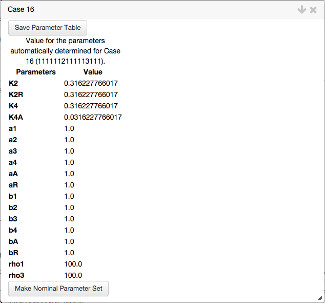
In this example we will use Case 16 as our phenotype of interest.
We select the
Analyze Casetab in theActionssub-menu of theMain Menutab, and input our selected phenotype, and press theCreate Analysisbutton.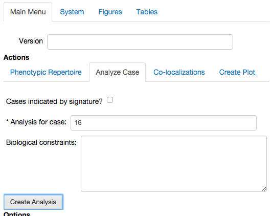
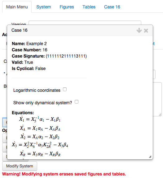
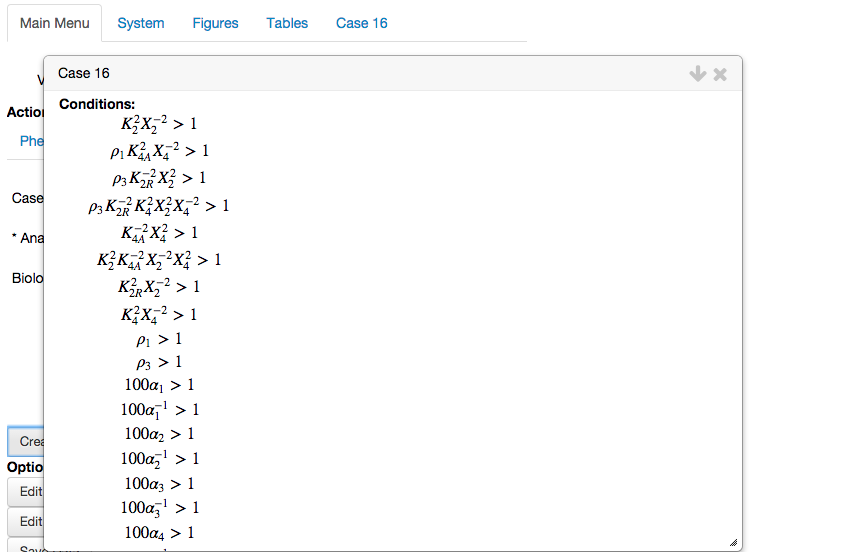
This opens the analysis report for the chosen phenotype, showing equations, solution, etc.
We scroll to the bottom of the report, and select the button called
Determine values for the parameters.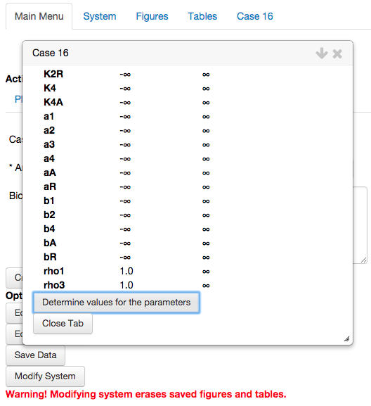
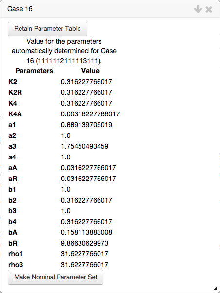
By selecting the Determine values for the parameters option, the toolbox automatically generates a set of parameter values in the interior of the feasible region. The set of values for the parameters for this representative point is represented in a table,
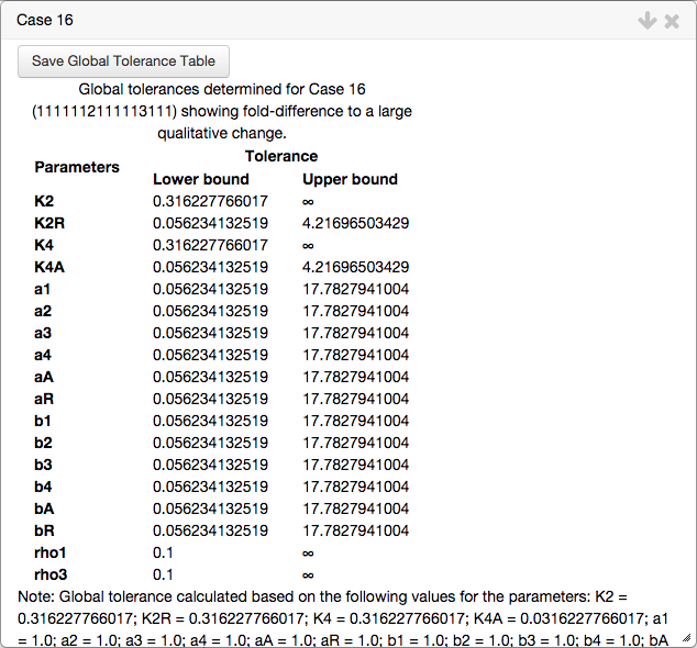
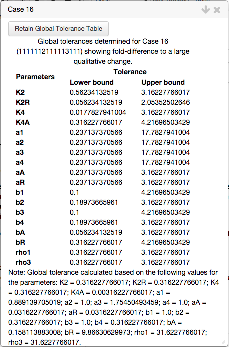
In addition, a second table is created showing the global tolerances from that point. The global tolerance indicates the fold-difference required for a qualitative change in system behavior, such that the phenotype of interest is no longer valid. The table showing the global tolerance for the automatically determined point s shown below,
Both tables can be added to the Tables tab in the top bar by clicking the corresponding Save Table button, which also saves the progress of the current project.
Local analyses about the automatically determined values for the parameters
The widget interface uses an internal parameter set that serves as a reference point for its plotting utilities. When paired with the automatically determined parameter values for a given case, it allows us to (1) visualize the phenotypic context (i.e. the phenotypes that surround the case of interest), (2) look at the local stability of the fixed points, (3) identify global topological structures such as hysteresis and global bifurcations and (4) visualize the steady-state concentration for species of interest.
At the bottom of the table showing the automatically determined values for the parameters, we select the option to Make Nominal Parameter Set,
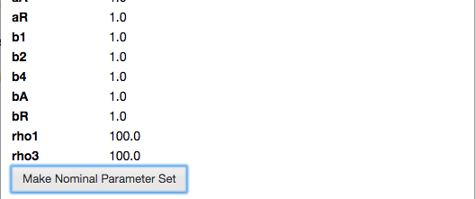
which copies the values of the parameters for this case and assigns them to an internal parameter set used for plotting.
Once the values for the automatically determined values for the parameters have been assigned to the internal set, we generate a design space plot using the Create Plot tab of the Main Menu.
Design Space Plot
The design space plot is created by selecting \(\beta_2\) and \(\beta_4\) as x-axis and y-axis, respectively; setting the * Plot Type option to Design Space; set the range for the x-axis and y-axis to 0.001 and 1000; and we center the plot on the internal parameter set by selecting the Center Axes option,

Note that the widget automatically creates a simple title and caption. Also, the default value for the # of intersections option is set to Single and three, which indicates that it will only show regions corresponding to individual cases and overlaps of three cases. In some cases, there are regions of overlap of more than 3 cases, or regions of overlap of 2, that are significant - in which case, this option should be set to All.
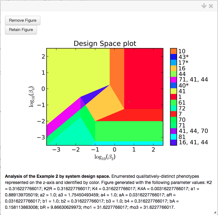
We select the Add Plot option, which opens a pop-up window showing the design space plot, the corresponding title and figure caption,
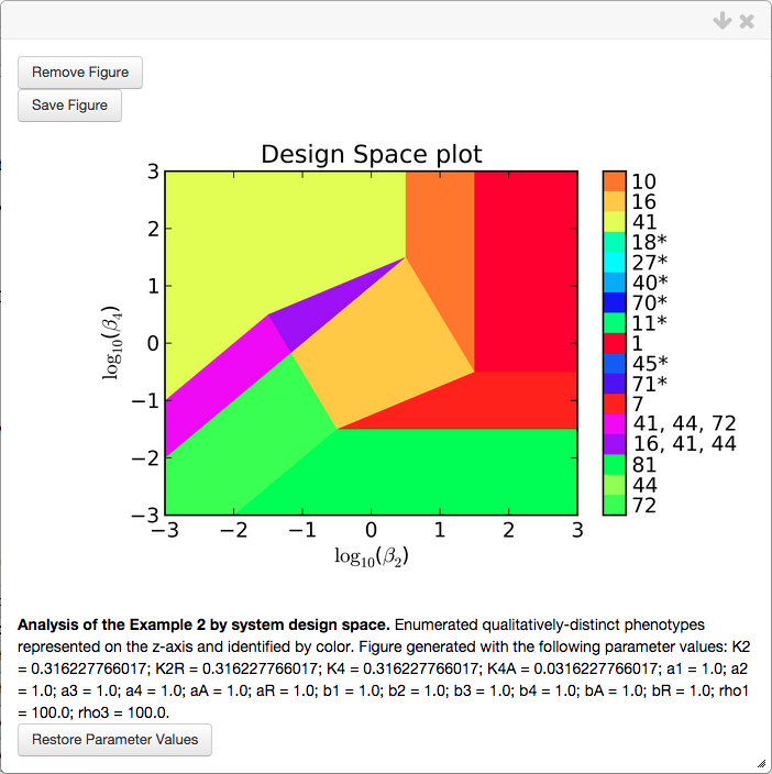
Note that the values for the parameters that were used to generate this plot are added to the caption. In addition, there is a button to Restore parameter values, which copies the values used for the plot to the internal parameter set.
The figure created is automatically added to the Figures tab of the top bar, under the header "Figures that will not be saved:". These figures are will not be saved by pressing the Save Data option in the Main Menu. Selecting the option to Save Figure moves them out of this section, assigns them a unique figure number, and saves the widget data. The images created by the toolbox are PNGs that can be copied by dragging the image directly to Word (or another word processor), dragging and dropping into a folder or desktop (on Mac OS X) or right-clicking the image and selecting the Save Image As... option.
Each region of the design space plot corresponds to a different phenotype of the system, or to an overlap of multiple phenotypes, as indicated by the key shown in the colorbar. Inspection of the colorbar reveals that there are more regions than what can be seen in the plot itself, many of the cases in the colorbar are shown with an asterisk and some regions have multiple cases, seperated by a comma.
The asterisks indicate cases that are marginally valid, meaning that the plot is showing either a 1-D face (i.e. a line) or a 2-D face of th evalid region. Thus the a infinitesimal change in one or more of the parameters can result in the loss of validity for that case. In this case, many of the parameters have a value of 1 and thus the left-hand side and right-hand side for many of the boundaries for case validity are equal (e.g. inspection of the boundaries for Case 7 shows that if all the parameters are equal to 1, both sides of all the inequalities are equal).
The regions corresponding to multiple cases seperated by commas are indicative of regions of overlap, where multiple cases are valid in the same region of design space. These regions provide information regarding the global topological structures of the system such as regions of multi-stability or global bifurcations. These global behaviors can be determined by analyzing the stability of the fixed points, which can be determined using a stability plot.
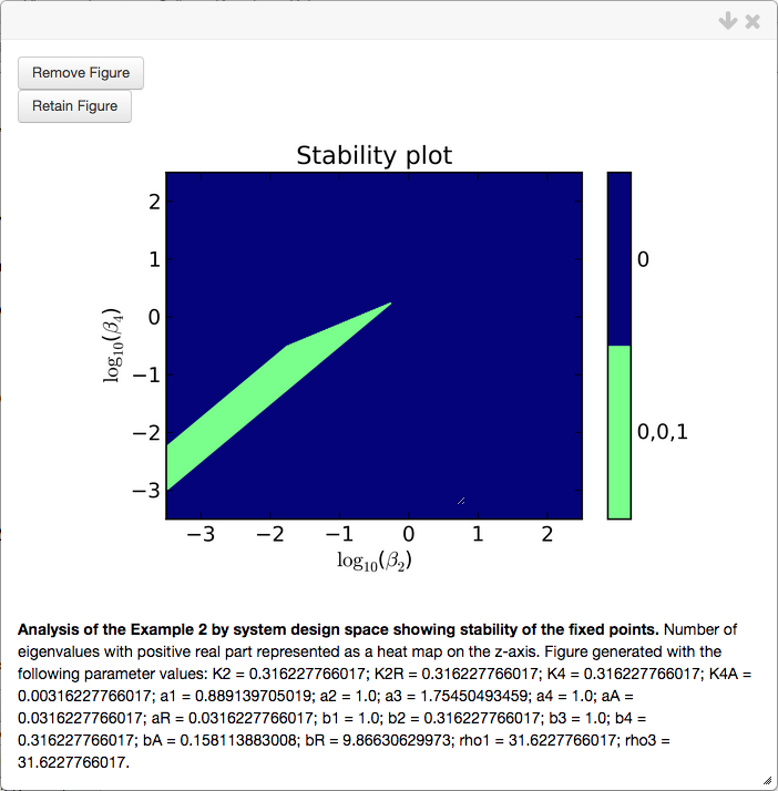
Stability Plot
The stability plot shows the number of eigenvalues with positive real part, and can be created through the Create Plot tab of the Actions sub-menu by selecting theStability plot type.
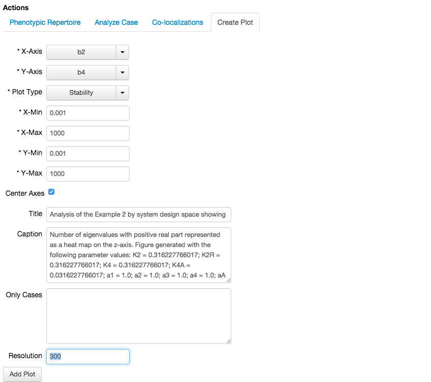
Note that by changing the plot type, we also change the menu inside the Create Plot tab, where instead of showing # of intersections, we now see Resolution. The stability of the fixed points is determined by sampling a grid of \(n\times n\) points, where \(n\) is the value of the Resolution field, and determining the stability for the fixed points for each phenotype valid at that point.
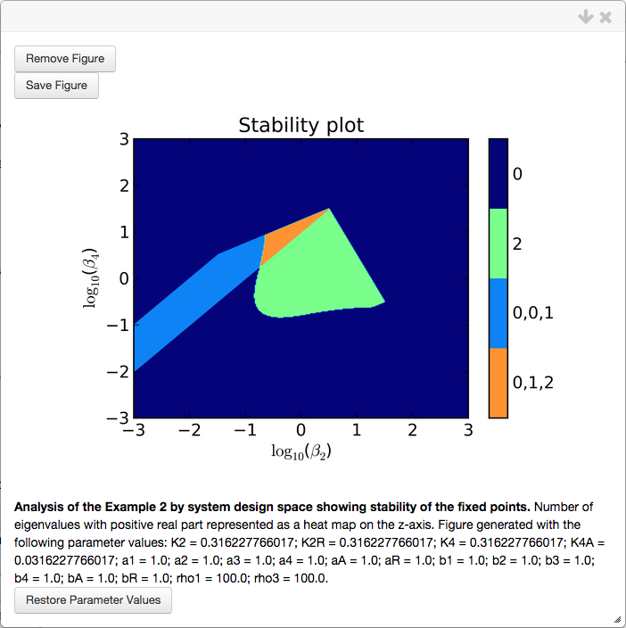
The stability plot for this system shows 4 distinct regions, two with a single fixed point and 2 with 3 fixed points. The regions with a single fixed point are either regions that are monostable (0 eigenvalues w/ positive real part) or exhibit the potential for limit cycle oscillations (2 eigenvalues w/ positive real part, i.e. a complex conjugate pair). Regions of overlap correspond to regions of bi-stability (two regions with 0 eigenvalues w/ positive real part, one with 1 eigenvalue w/ positive real part) and regions that give rise to a saddle-node into limit cycle bifurcation (SNIC) - as is the case in this example.
In addition to stability plots, we can plot the steady-state concentration, fluxes and arbitrary real-valued mathematical functions involving the parameters, concentration and fluxes. These plots will not be covered in this section.
Automatically determined 'biological' values for the parameters.
We can repeat the steps to automatically determine values for any of the cases within specific ranges for the parameters. We achieve this by following the same series of steps as in the second sub-section, but instead add biological constraints in Step 2. We reiterate the steps here,
Choose a phenotype of interest from the phenotypic repertoire.
Again we choose Case 16 as our phenotype of interest.
We select the
Analyze Casetab in theActionssub-menu of theMain Menutab, and input our selected phenotype, and enter constraints that limit the values of the parameters to biological ranges, we then press theCreate Analysisbutton.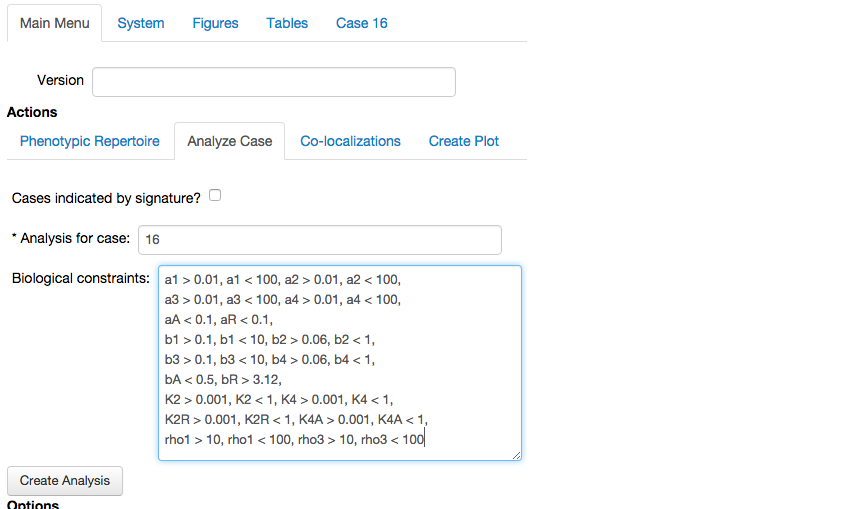
This opens the analysis report for the chosen phenotype, this time with the biological conditions and boundaries.
We scroll to the bottom of the report, and select the button called
Determine values for the parameters.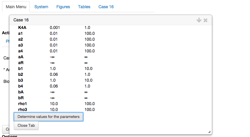
By selecting the Determine values for the parameters option, the toolbox automatically generates a set of parameter values in the interior of the feasible region within the constraints we have defined as biologically relevant. Again, the toolbox displays a table with the automatically determined values for the parameters,
and a table showing the global tolerances of the automatically determined value for the parameters, which includes the tolerance to the biological constraints,
As with other tables, both tables can be saved and added to the Tables tab in the top bar by clicking the corresponding Save Table button.
The automatically determined values for the parameters within what we have designated as biologically relevant can be copied and used as the nominal set. By using these values we get a new design space image,
and corresponding stability plot,
Jason G. Lomnitz
Savageau Lab
Department of Biomedical Engineering
University of California
Davis, CA 95616
jlomn@ucdavis.edu