Previous Section Table of Contents Next Section

Design Space Toolbox Preliminaries

Technology Overview

The design space toolbox V2 is a high performance software package that enables analysis of mathematical models by means of the design space method (Savageau, 2009). This software library is the second iteration of the design space toolbox, originally written by Rick Fasani in Matlab® (Fasani, 2010).

This version of the design space toolbox provides multiple improvements addressing performance and usability and expands its capabilities to include recent developments in the design space methodology (Lomnitz, 2013; Lomnitz, 2015). It also addresses the issue of accesibility by being built entirely on open-source software.

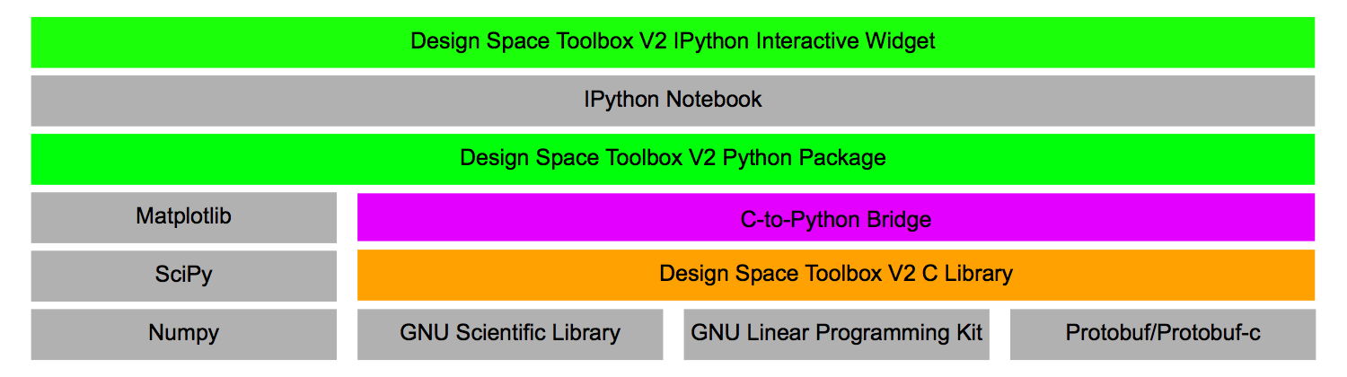
The design space toolbox V2 - from here on referred to simply as "the design space toolbox" - provides a large collection of tools that automate the difficult steps of the design space method within an interactive scientific programming environment. The toolbox achieves high performance and multi-threaded parallelization together with interactivity thanks to a hierarchical implementation involving compiled and interpreted components, written using multiple programming languages, as represented visually in the figure below.

**Technology Overview of the design space toolbox V2.** Components are represented by rectangles, stacks represent component dependencies. Different component types are represented by color: C library (orange); Python packages (green); and C/Python wrapper (purple); and third-party dependencies (gray).

This workshop will focus exclusively on the top-level of the design space toolbox involving graphical user elements, known as widgets, that are running inside an IPython notebook environment. At this level, the design space toolbox provides much of the functionality available, while remaining accessible to a larger community with limited python programming experience. For users with more programming expertise, the data associated with the widgets can be extracted and more complex tasks can be carried out using the Python package.

Installing the Design Space Toolbox V2

Installation Preamble

The following sub-section will go over the installation of the design space toolbox and its dependencies on either Mac OS X Yosemite or Ubuntu GNU/Linux. In addition, a virtual hard drive with the toolbox installed with the latest version of this toolbox as of the date of the workshop is provided for use with VirtualBox.

This section will cover installation of the following components:

The design space toolbox V2 C library

The C toolbox is currently accesible via a private repository and is accessed through your bitbucket account (you should have received an e-mail from bitbucket granting you access).
The design space toolbox V2 dspace Python package

The dspace Python package is available via a public repository.
The design space toolbox update script

This script downloads and manages the installation of both the C toolbox and the dspace Python package. It easily updates the toolbox and to switch back-and-forth between release and development versions.

Including the dependencies of the Design Space Toolbox C library:

The GNU Scientific Library [gsl]
The Protocol Buffers Library [protobuf]
The Protocol Buffers in C implementation [protobuf-c]
The GLPK library modified for thread safety [glpk]

the dependencies of the dspace Python package:

and the dependencies of the IPython Notebook interactive widgets:

IPython 2.2.0 (with the Notebook components)

The instructions for installing the toolbox on Mac OS X and Ubuntu assume that the user is a system administrator. Installation may take 30-45 mins to complete.

Mac OS X Yosemite

The following shows the necessary steps to install the toolbox and its dependencies on a system running Mac OS X Yosemite. Installation on Mac OS X is simplified because many of the dependencies are included with the operating system.

Setting up your Mac OS X system

To install the design space toolbox, we need the command line developer tools installed. To test if the tools are available, try the following command in a new terminal window (the $ is used to indicate the command prompt and should not be included):

$ gcc

if gcc is available, the terminal should output

clag: error: no input files

otherwise, a dialog box will appear with the option to install the tools.

Once the developer tools are installed, we proceed to install the homebrew package manager. This package manager will simplify the steps needed to setup the remaining dependencies.

To install homebrew, copy and paste the following command at the terminal prompt:

$ ruby -e "$(curl -fsSL https://raw.githubusercontent.com/Homebrew/install/master/install)"

and follow the instructions, as they appear.

Installing the dependencies for the C toolbox

With homebrew installed, we install the GNU scientific library, pkg-config and wget:

To install GSL:

$ brew install gsl
$ brew install pkg-config
$ brew install wget

The last remaining dependencies of the C toolbox, protobuf and protobuf-c, must be installed from source. The following commands will (1) download the source code, (2) unpack it and (3) install it.

For protobuf, copy and paste the following block into the terminal:

cd ~/Downloads
wget https://github.com/google/protobuf/releases/download/v2.6.1/protobuf-2.6.1.tar.gz
tar -xvf protobuf-2.6.1.tar.gz
cd protobuf-2.6.1
./configure && make && sudo make install

Next, copy and paste the following block into the terminal after to install protobuf-c:

cd ~/Downloads
wget https://github.com/protobuf-c/protobuf-c/releases/download/v1.1.1/protobuf-c-1.1.1.tar.gz
tar -xvf protobuf-c-1.1.1.tar.gz
cd protobuf-c-1.1.1
./configure && make && sudo make install

Installing the C toolbox and dspace Python package

To install the design space toolbox, type the following command in the terminal by replacing <user_name> with your bitbucket username,

$ bit_username=<user_name>

then copy and paste the following blocks into the terminal:

cd
curl https://bitbucket.org/jglomnitz/toolbox-update-script/raw/v1.2.0/toolbox_update.py -O
chmod +x toolbox_update.py
./toolbox_update.py --update-script

cd Documents
git clone https://$bit_username@bitbucket.org/jglomnitz/design-space-toolbox.git
cd

sudo ./toolbox_update.py --stable --glpk-dependency

At any time, the toolbox can be updated using the following command in a terminal window,

# This is not necessary after installation, 
# the toolbox will already be up to date.
$ sudo ./toolbox_update.py --stable

Installing IPython and the IPython Notebook components

Installation of the ipython notebook is done through the pip python package manager. To install pip, use the following command in the terminal window:

$ sudo easy_install pip

and then install the ipython notebook v2.2.0:

$ sudo pip install ipython[all]==2.2.0

Ubuntu GNU/Linux 15.04

The following shows the necessary steps to install the toolbox and its dependencies on a system running Ubuntu. This example assumes Ubuntu 15.04, but the process should be the same for other versions.

Open a terminal window and ensure that the package manager is up to date by typing in the following command,

$ sudo apt-get update

then, open a plain text editor, such as gedit, and create a new file. Save it as install_toolbox.sh in the home directory.

Copy the following script,

#!/bin/sh
export LD_LIBRARY_PATH=/usr/local/lib:$LD_LIBRARY_PATH

read -p "Enter bitbucket username:" bit_username

# Installing
sudo apt-get install curl libatlas3-base libatlas-dev libgsl0-dev git libpython2.7-dev python-numpy python-scipy python-matplotlib python-pip ipython-notebook

cd ~/Downloads
wget https://github.com/google/protobuf/releases/download/v2.6.1/protobuf-2.6.1.tar.gz
tar -xvf protobuf-2.6.1.tar.gz
cd protobuf-2.6.1
./configure && make && sudo make install

cd ~/Downloads
wget https://github.com/protobuf-c/protobuf-c/releases/download/v1.1.1/protobuf-c-1.1.1.tar.gz
tar -xvf protobuf-c-1.1.1.tar.gz
cd protobuf-c-1.1.1
./configure && make && sudo make install

sudo ln -s /usr/lib/libcblas.so.3 /usr/local/lib/libcblas.so
sudo ln -s /usr/lib/libgsl.so /usr/local/lib/libgsl.so
cd
curl https://bitbucket.org/jglomnitz/toolbox-update-script/raw/v1.2.0/toolbox_update.py -O
chmod +x toolbox_update.py
./toolbox_update.py --update-script

cd Documents
git clone https://$bit_username@bitbucket.org/jglomnitz/design-space-toolbox.git
cd

sudo ./toolbox_update.py --stable --glpk-dependency
# End Install Script

and paste it into the text editor, save the file and close it.

In the terminal, type the following commands,

$ cd
$ chmod +x install_toolbox.sh
$ ./install_toolbox.sh

and the program will run, prompting the user to confirm the packages that will be installed, indicate the bitbucket username, butbucket password and your user's password. Completing this step should automatically install all the dependencies, the toolbox C library and the python components.

At any time, the toolbox can be updated using the following command in a terminal window,

# This is not necessary after installation, 
# the toolbox will already be up to date.
$ sudo ./toolbox_update.py --stable

VirtualBox Ubuntu 15.04 VM Image

The last option is to download a virtual hardrive for VirtualBox running Ubuntu 15.04. This virtual hardrive has the design space toolbox pre-installed. This option is best for Windows users, users of other distributions of linux or those that experience difficulties during the installation process. To use the Virtual hardrive:

Download and install VirtualBox.
Download and install VM VirtualBox Extension Pack.
Download the Workshop Ubuntu 15.04 virtual hard disk file.
Create a new virtual machine, with a desired name, of type Linux, with version Ubuntu (64-bit).
Select the amount of memory for the virtual machine.

The design space toolbox can exhaust system memory for larger problems. However, for the purpose of the workshop amount of memory does not need to be very large.
Select the option to Use an existing virtual hard disk file and select the Workshop Ubuntu 15.04 virtual hard disk file.
Start the virtual machine.
Log into the computer with the following information:
```
User: Workshop
Password: bstconf14
```

This workshop will show the capabilities of the design space toolbox via a graphical user interface built on widgets embedded in the IPython Notebook (Pérez, 2007).

The ipython notebook is initialized by typing the following command in a terminal window,

$ ipython notebook

this opens a browser window with the IPython notebook home screen.

We select the New Notebook option in the top-right corner of the navigation window. This will open a new tab in the browser showing a new IPython notebook.

The design space toolbox widget interface is loaded into the Python environment by typing the following command inside a code cell in the new notebook,

from dspace.display.UI.interactive_input import InteractiveInput

Notice that the above statement is inside a gray box with a In [1]: statement on the left margin. These indicate Code cells within the IPython notebook. New code cells can be added by selecting Insert → Insert Cell Below from the IPython notebook menu bar. After inserting a command in a code cell, as shown above, the cell needs to be run by selecting Cell → Run from the IPython notebook menu bar, while the cursor is inside the code cell; or, alternatively by pressing the

button in the IPython notebook toolbar.

The InteractiveInput widget is used to input the model equations and analyze it via the design space method. For the purpose of illustrating the widget interface, we use a very simple example involving two chemical species, represented by the variables $X_1$ and $X_2$, shown by the following diagram,

where each arrow represents a chemical reaction that results in synthesis or loss of either $X_1$ or $X_2$. The $\hat{X}_3$ and $X_4$ are independent variables that represent inputs into the system. The $\hat{}$ symbol on $X_3$ does not hold any specific meaning, but will be used to illustrate the typesetting capabilities of the interactive widget.

The mathematical model is given by the following system of equations,

$\frac{d X_1}{d t} = \alpha_{11} + \alpha_{12}\hat{X}_3 + \alpha_{13}X_4 - \beta_1X_1$ $\frac{d X_2}{d t} = \beta_1X_1 + \alpha_{21} - \beta_2 X_2$

Creating a system design space

The following sub-section provides a graphical overview of the widget user interface. To initiate the widgets, we create a new InteractiveInput object.

example_1 = InteractiveInput()

The InteractiveInput object spawns a menu with two fields: Name and Version. In addition, there are 2 buttons: Create Design Space for a new design space and Load Data to open an existing project as determined by the Name and Version fields.

The Name field designates the name of the project, and the Version field is used to create alternative saved files for the same project that can be loaded individually.

Leaving the Version field blank when creating a design space project indicates that no versioning has been establshed. When loading a design space with an empty Version field tells the program to load the latest version of the project.

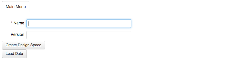
Note that the Name field has an asterisk that preceeds it. Asterisks are used to indicate fields that are mandatory.

In this example, we create a new design space project, with Name 'Example 1' and selecting the Create design space option. The result is an expanded menu where the model can be input into the toolbox widget.

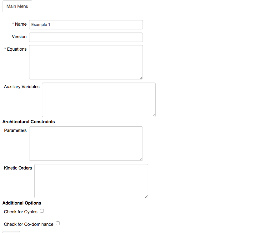
Here we input the model described above by representing each of the equations by a string,

and select the Done button to proceed with the analysis.

Note that the system used in this section is very simple and we did not need to specify values for any of the field other than the Equations. A detailed treatment of model formulation will be disccused in Section II.

After creating the design space, a simple menu appears with different tabs along a top bar. The first tab in the top bar is reserved for the main menu, and all remaining tabs in the top bar are used to display information of different properties of the system, and/or results of analyses performed within the widget.

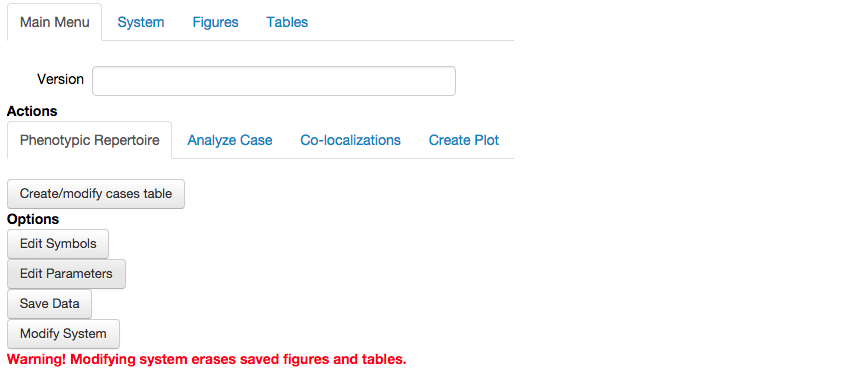
The Main Menu tab is the starting point for any project, and is used to (1) perform different analyses and (2) modify different properties of the design space project.

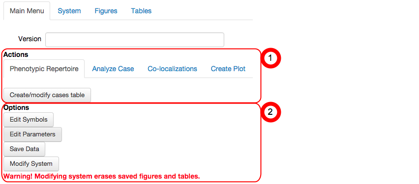
Actions

The Actions sub-menu contains tools to analyze a model and will be the primary focus of this workshop. The first three tabs: (1) Phenotypic Repertoire, (2) Analyze Case and (3) Co-localizations will be discussed in detail in Sections III, IV and V, respectively. The Create Plot tab will be used throughout the workshop and thus we discuss briefly here.

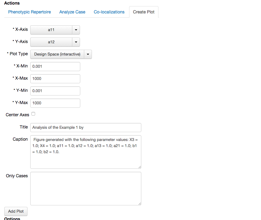
Creating plots

The Create Plot tab provides a menu used to define a particular plot among a variety of plot types. These include design space plots, plots showing the stability of the fixed points, steady-state concentrations, fluxes and other mathematical functions. The menu allows for the user to specify the variables on the x- and y-axes, the range of the axes, type of plot, etc.

Options

The Options sub-menu includes utilities to modify properties of the current project.

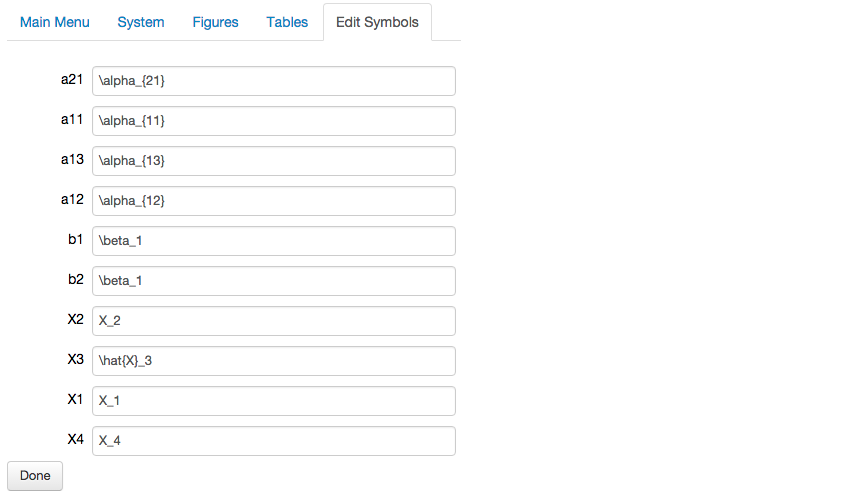
The Edit Symbols button is used to specify the latex notation for variables and parameters of the model. The latex notation is used throughout the widget to typeset all equations and constraints using mathematical symbols. Latex notation for a large number of mathematical symbols can be found here.

The latex notation for the symbols for the simple model we input to the design space toolbox are specified as follows:

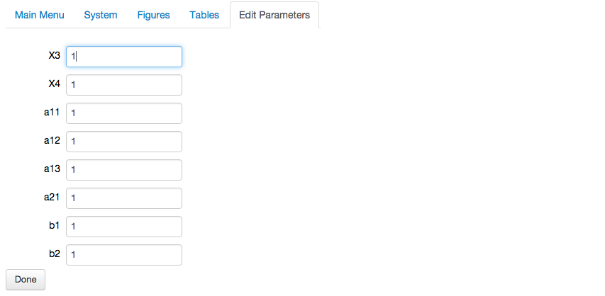
The Edit Parameters button is used to manually change the values for individual parameters and independent variables. Here, we emphasize that this is optional, given that the design space method provides many tools to automatically determine values for the parameters. In fact, at no point in this workshop will we manually enter values for any of the parameters.

The Save Data button is used to save the results of the analysis. This can be done at any point in time by pressing the Save Data button, and by changing the version information in the Version field. One can always return to a previous version by specifying the version and selecting the Load Data option in a new widget.

Top-bar tabs showing system information and results of the analyses

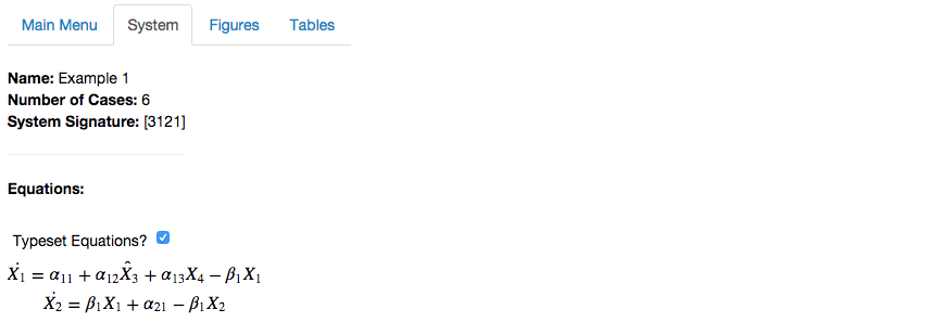
The System tab displays important information for a particular system. The information that is displayed includes the maximum number of possible qualitatively-distinct phenotypes, the system signature and the system equations, typeset using the mathematical symbols as defined by the latex notation.

The Figures tab displays figures generated using the Create Plot tab of the Main Menu. Similarly, the Tables tab displays tables that are generated from one of the many analyses results. Tables must be saved for them to appear in the Tables tab, which is achieved by pressing the Save Table button that appears above tables generated in the widget. Both the Figures and Tables tabs are empty when starting a new project. This birds-eye view of the widget interface will be made much clearer as we explore the functionality of the design space toolbox widget interface.